Tutorial 15: Variable Retirement and Servicing

Motivation

In prior tutorials, we mentioned that a 5% retirement rate corresponds to a 20 year average lifespan. However, in practice some equipment will retire before 20 years and some after. That in mind, how does Kigali Sim actually interpret that 5% directive? In survivor analysis, we specifically say that this is a constant "hazards rate" meaning that, each year, each unit of equipment has a 5% chance of retiring. In practice, this makes sense for many countries which may not know the specific age of equipment already in service or might not have a good estimate for how the rate of failure changes over time. With few assumptions, we still get realistic dynamics like a long tail of equipment on phase out and some retirement prior to the amortized lifespan estimate.

All that said, Kigali Sim can take in more sophisticated estimates if available. In this tutorial, we will create a hazard rate which changes according to the age of equipment in a simulation that reaches back to 1990 which we assume to be the first year in which the equipment we are studying appeared within the country. Then, for those with just a little extra modeling background, we will optionally make a more sophisticated model to fit some information one might have about equipment even if maybe you don't know the exact hazard function.

This tutorial will use the QubecTalk code-based editor. However, you can enter in formulas through the UI-based editor as well! Instead of providing a single number for retirement or recharge, enter your formula instead.

Using default assumptions

Before we consider the complex lifecycle, let's set up a simplier simulation in which we model HFC-134a (1 kg / unit initial charge and no servicing). In order to observe how retirement works, let's have 1990 with one million (1,000,000) units of equipment sales but no sales in 1991 onwards. Let's assume a 5% retirement rate and simulate a business as usual scenario from 1990 to 2020.

We see that equipment does drop but, if we took the 5% as 20 year lifespan seriously, we wouldn't have any population (see bank and set to units of equipment) after 2010. Instead, we see that some equipment keeps "getting lucky" and surviving that annual retirement probability (hazard rate) of 5%. This is like how you aren't guaranteed to have a heads on a coin after two flips.

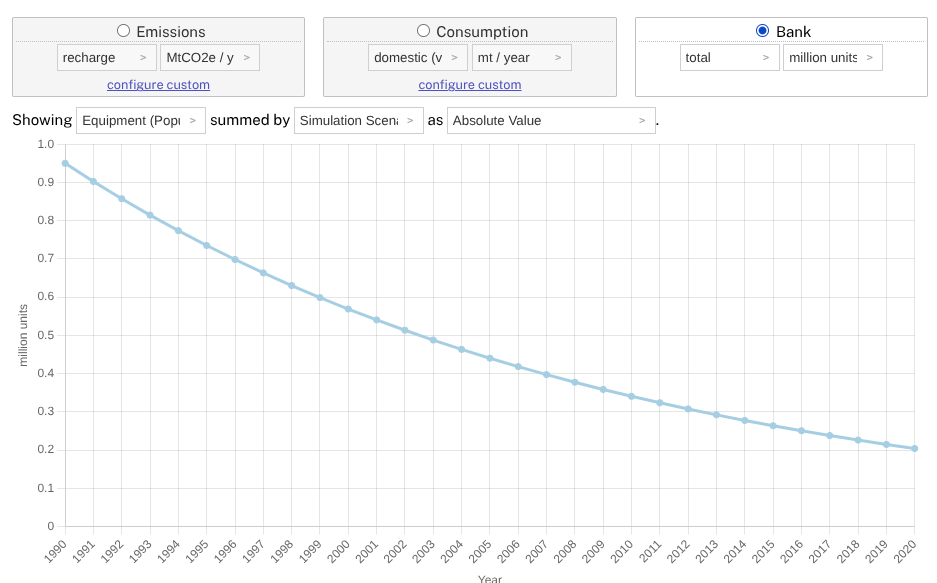
To see this effect, please have bank selected with units of equipment.

Increasing hazard rates with age

In some ways, this lingering population of equipment actually reflects what we would expect, especially if a substance suddenly became no longer available. However, let's change this hazard rate such that the probability of failure is 1% multiplied by the age of the equipment in years. So, 1% at 1 year, 2% at 2 years, and so on. To do this, modify the simulation using QubecTalk code like follows:

uses substance "HFC-134a"
  enable import
  initial charge with 0 kg / unit for domestic
  initial charge with 1 kg / unit for import
  initial charge with 0 kg / unit for export
  equals 1430 kgCO2e / kg
  equals 1 kwh / unit
  set priorEquipment to 1,000,000,000 units during year 1990
  retire (get age as years) * 1 % / year
end substance

By the time we get to 2000, much of the equipment is already a few years old so its hazard rate is already higher than the 5% we previously assumed. This rate keeps going up as our population of equipment ages, causing us to hit zero units much sooner.

Download the completed tutorial: tutorial_15.qta which contains the complete variable retirement model with age-dependent hazard rates. If you are using the UI-based editor, you can instead enter "(get age as years) * 1" into the text box for retirement (without quotes)!

Fitting a function (optional)

In our first example, we assumed we already knew the hazard function: a specific estimate of how much we expect the probability of retirement (or servicing) to change with equipment age. This captures some important real-world dynamics! However, some users might not have that detailed information.

Let's consider a second optional example. For those with just a little calculus or maybe some background in operations research or reliability engineering, let's address a slightly more messy situation where maybe we have some basic data about equipment but not an exact hazard function. Specifically, let's assume:

• We have about an average 10 year lifespan or, more precisely, we find that a unit has about a 50% chance of having retired by the end of 10 years of service.
• We believe that the probability of retirement increases exponentially with age.
• Equipment leak about 6% of initial charge over 10 years or, more precisely, equipment still in service at year 10 will have leaked around 6% of their initial charge.
• We service to top up to original charge.
• We believe that leakage increases linearly with age.

With these constraints in mind, we can approximate using the following:

start default

  define application "MAC"
  
    uses substance "HFC-134a"
      enable import
      assume only recharge sales
      initial charge with 0 kg / unit for domestic
      initial charge with 1 kg / unit for import
      initial charge with 0 kg / unit for export
      equals 1430 kgCO2e / kg
      equals 1 kwh / unit
      set priorEquipment to 100 units during year 2020
      retire (get age as years) ^ 2 * 3 / 2000 * 100 % / year
      recharge (get age as years) * 3 / 2500 * 100 % with 1 kg / unit
    end substance
  
  end application

end default


start simulations

  simulate "BAU"
  from years 2020 to 2040

end simulations

How did we arrive at those formulas? Here, we need that tiny bit of calculus. We can integrate over the first ten years of life such that we have 50% retirement and 6% recharge. With this operation, we derive a hazard function to fit observed data! Consider the following short code snippets runnable at Wolfram Alpha:

• Solve for retirement rate: integrate x*t^2 from t=0 to 10 equals 0.5, solve for x.
• Solve for servicing: integrate x*t from t=0 to 10 equals 0.06, solve for x

These are provided in Wolfram Alpha for brevity but can be adapted easily to Python (using numpy) or other languages. The point here being though that we assume retirement gets exponentially worse with age and leakge linearly worse. If you have some programming background, you can also use a numeric solver with a summation in addition to this approach!

Note that we are providing a very direct interpretation of the input assumptions. For some alternative types of input, consider using numpy / Python and an iterative solver. Also, Kigali Sim applies calculations once per year as we don't know the exact time during the year that equipment comes into service. So, in actuality, we pass the 50% mark sometime between 2030 and 2031. Emissions might also be slightly different.

Conclusion

If you have survival analysis data and detailed information on the age of equipment, specifying variable retirement may lead to higher accuracy in predictions. Additionally, though we looked at hazard rates for retirement, the same approach can apply to servicing as well.

All that said, maybe the calculus option feels a little out of reach mathematically or maybe just a tad too much for a quick analysis. This is a very advanced approach! Even providing a simple age-dependent formula can get you most of the way there. Adding in some of these dynamics can help better align your predictions to reality, particularly if your equipment population is small or only very recently sold.

Even so, consider if you really know the likely age of existing equipment or a specific schedule for retirement. If not, it may still be best to stick to a flat percentage retirement per year. This simple approach is often most honest when those detailed data aren't available or perhaps the estimates might be less reliable. There is no shame in going with a flat percentage, especially early in modeling.

Finally, please note that, in this tutorial, we still specify hazard rates (rates of retirement) as a percentage. However, you can also specify an absolute number of units of equipment or volume equivalent (kg, mt, CO2e) to retire each year.

Next Steps

You've learned how to leverage sophisticated features like variable retirement rates, bank-based modeling, and advanced sales assumptions. In the next step, we look at Monte Carlo.

Previous: Tutorial 14 | Return to Guide Index | Next: Tutorial 16